The dispersive material calculator finds Debye-Drude parameters that fit measured data and constant loss tangent by using optimization.
Dispersive Material Calculator | XFdtd
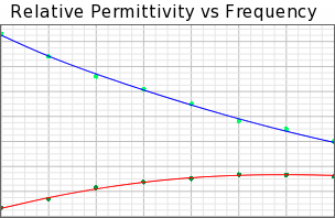
![]() Fit a Debye-Drude material to measured data.
Fit a Debye-Drude material to measured data.