Corner Reflector – WaveFarer

The radar range equation is commonly used as an analytic tool that calculates the received power for a target at a specified distance from a transceiver.

\begin{equation} P_r = P_tG_tG_r\left(\frac{\lambda}{4\pi R}\right)^2\frac{\sigma}{4\pi R^2} \end{equation}

This equation can be solved for multiple distances and plotted for comparison. WaveFarer produces the same results at the radar range equation, as demonstrated in this tutorial.

In this tutorial, a transceiver consisting of one transmitter and one receiver uses 24.1 GHz antennas with 16 dBi gain and transmits 0 dBmw of power. The received power for a 20 dBsm corner reflector at incremented distances between 5 and 160 meters is simulated, and then graphs WaveFarer's generated results against the radar range equation.

This tutorial utilizes the following skills:

Creating a corner reflector by defining a pyramid.
Defining a parameter that varies the distance between the corner reflector and the origin.
Assign a PEC material to the corner reflector in order to define its electromagnetic properties.
Adding two transceiver components, each including a 45 degree directional antenna: one transmitter with a waveform frequency of 24.1 GHz and one receiver.
Setting the analysis configuration to include 2 reflections, 1 diffraction, facet targeting, and MEC diffractions.
Writing and executing a script that animates the geometry and confirms correct parameter sweep behavior.
Running a simulation that performs a parameter sweep from 5 to 160 meters with a 2.5 meter increment.
Evaluate the received power versus its distance from the origin.
Import a script that plots the radar range equation.

Step 1: Create the Geometry

The corner reflector will be modeled as a hollow pyramid, and then oriented to face the transmit and receive antennas. The remove faces feature will turn the pyramid into the desired corner reflector with three sides.

First, create the part.

Right-click on Parts in the Project Tree and select Create New ❯ Pyramid to open the editor.
Under the Edit Pyramid tab, define its size by typing in (.247 m) / sqrt(3) as the Height value.
Enter (.247 m) * sqrt(2/3) as the Radius 1 value.
Enter (.247 m) * sqrt(2/3) as the Radius 2 value.
Enter 0 m as the Top value.
Enter 3 as the Sides value.
Select Sheet using the Create as drop-down arrow.
Enter the geometry name by typing Corner Reflector into the Name field.
Under the Specify Orientation tab, select YZ Plane from the Presets drop-down menu.
In the Geometry window, right-click on the W axis and select Rotate around W'.
Enter -90 deg.
Click Done in the upper-right corner of the window to close the editor.

Then, remove one of the faces.

Right-click on the Corner Reflector in the Project Tree, then select Modify ❯ Remove Faces.
Click the Zoom to Extents button in the right sidebar.
Click on the face in the YZ plane.
Under the Preview tab, uncheck Close gaps left by removed faces.
Click Done to close the editor.

Step 2: Parameterize the Corner Reflector

A parameter can be defined as a single value or formula, and can then be used in most of WaveFarer's edit fields. In this example, we will use parameterization to move the corner reflector along the x-axis.

First, create a parameter.

Click the Parameters button on the right side of the WaveFarer window.
Click the button in the upper-left corner of the Parameters window.
Enter the parameter name by typing targetLocation into the highlighted field.
Press Tab and type 10 m into the Formula cell.
Press Tab and type Distance to the corner reflector into the Description cell.
Click Apply.

Then, apply the parameter to the the reflector.

Right-click on the Corner Reflector in the Project Tree and select Modify ❯ Transform ❯ Translate.
Under the Specify Translation tab, click and drag the W' arrow to verify that the Corner Reflector moves along the x-axis.
Enter targetLocation as the W' value.
Click Done to close the editor.

View the corner reflector's new coordinates in the bounding box of the Geometry window by clicking the Zoom to Extents button and then clicking on the Corner Reflector in the Project Tree. Verify that the Corner Reflector moves according to the parameter's Formula by changing the definition to 15 m in the Parameters window, clicking Apply, and rechecking the bounding box.

Step 3: Define and Assign a PEC Material

A material needs to be associated with the geometry in order to determine its scattering behavior, so a material first needs to be defined and then assigned to the corner reflector. WaveFarer's definitions node allows users to define a set of electromagnetic properties once and use it in multiple places, although this tutorial is basic and requires just one.

First, define the reflector material.

Right-click on Materials in the Project Tree and select New Material Definition.
Enter the New Material name by typing PEC into the Project Tree.
Press Enter to commit the change to the project.
Double-click on PEC in the Project Tree to open the Material Editor.
Change the Type to Perfect Electrical Conductor (PEC) using the drop-down arrow.
If desired, navigate to the Appearance tab and change the PEC material's display color.
Click Done to finish the PEC material.

Then, assign the material to the Corner Reflector.

Click and drag the PEC material from the Definitions branch of the Project Tree and drop it on top of the Corner Reflector in the Parts branch of the Project Tree.

Step 4: Create a Transceiver

The transceiver serves as the point where the rays are sent and received. For this tutorial, it will consist of one transmitter and one receiver with associated waveform and antenna definitions.

First, define the antenna.

In the Definitions branch of the Project Tree, right-click on Antennas and select New Antenna Definition.
Enter the antenna name by typing Directional (45 deg) into the Project Tree.
Press Enter to add the new antenna to the project.
Double-click on Directional (45 deg) in the Project Tree to open the Antenna Editor.
In the editor, click the Type drop-down arrow and select Directional.
Enter 45 degrees as the E-Plane Half Power Beam Width.
Enter 45 degrees as the H-Plane Half Power Beam Width.
Uncheck Auto and enter 16 dBi as the Maximum Gain.
Click Done to close the editor.

Next, create the transceiver.

Right-click on the Transceivers branch of the Project Tree and select New Transceiver Points Layout to open the editor.
Under the Layout tab, click in the Type field and use the drop-down arrow to select Transmitter.
In the next column, check the box that Activates the antenna pattern for viewing at this location.
Click Zoom to Extents in the right sidebar, then zoom in using the middle mouse wheel.
Check the Changes to Radius Affects All Points option.
Click in the Radius column and enter 0.02 m.
Click the button on the right side of the Layout tab.
Click in the second point's Type field and use the drop-down arrow to select Receiver.
Press Enter to apply the change.
Select the first point in the table by clicking on Transmitter.
Toggle the orientation-editing settings by clicking the button at the top of the tab.
Enter 0.02 m as the Y value.
Press Enter to apply the change.
Change the Point to 2 to select the Receiver.
Enter -0.02 m as the Y value.
Press Enter to apply the change.
Enter the transceiver name by typing Transceiver w/ 1 Tx, 1 Rx into the Name field.
Click Done to close the editor.

Then, set the waveform's properties.

In the Definitions branch of the Project Tree, double-click on the Sinusoid waveform to open the Waveform Editor.
Enter 24.1 GHz as the Frequency.
Enter the waveform name by typing 24.1 GHz Sinusoid into the Name field.
Click Done to close the editor.

Step 5: Set the Analysis Configuration

Users can enter inputs in the analysis configuration settings that control how the calculation engine evaluates the simulation space, modifying the tradeoff between accuracy and run time. The reflection and diffraction values determine the maximum amount of interactions a ray path can have with geometry faces and edges. Higher numbers increase accuracy, as well as run time.

Right-click on Analysis Configurations in the Project Tree and select New Physical Optics Configuration.
Enter the configuration name by typing 2R1D into the highlighted field.
Press Enter to add the configuration to the project.
Double-click on 2R1D in the Project Tree to open the Physical Optics Configuration Editor.

Under the Properties tab, the default settings are desired for this project. Confirm that the Number of Reflections is 2, Number of Diffractions is 1, Minimum Angular Ray Spacing is 0.01 degrees, Restrict Rays By Gain Threshold is checked with a value of 30 dBi, Include MEC Diffractions is checked, and Allow Knide Edges is unchecked.

Click Done to close the editor.

Step 6: Animate the Scenario

Once the project is set up, users can animate the geometry by writing and executing a short script. This step is not required, but it is recommended because it provides visual confirmation that the parameter sweep will behave as expected when the simulation is created.

Right-click on the Scripts branch of the Project Tree, then select New Macro Script to open the Scripting window.
In the Project Tree, right-click on New Macro Script and select Rename.
Enter the script's name by typing Sweep targetLocation into the Project Tree.
Press Enter to commit the change to the project.
Enter the following script into the Scripting window:

var list = App.getActiveProject().getParameterList();

for( var t = 5; t <= 160; t += 5 )
{
list.setFormula( "targetLocation", t + " m" );
App.sleep( 100 );
}

Save the script by clicking the Commit button in the toolbar, and close the Scripting window.

Place the geometry within view by clicking Zoom to Extents in the right sidebar.

Right-click on Sweep targetLocation in the Project Tree, then select Execute to run the script.

Watch the Corner Reflector move along the x-axis until it is outside of the Geometry view.

Step 7: Create and Run a Simulation

Once the project is complete, it must be saved in order to create a new simulation and write output files.

First, save the project.

Click File in the upper-left corner of the WaveFarer window, then select Save Project As.
Enter Corner Reflector as the project name.
Click Save.

Then, create and run the simulation.

Click the Simulations button in the upper-right corner of WaveFarer to open the Simulations window.
Click the Create New Simulation button in the upper-left corner of the Simulations window.
In the Create Simulation window, enter the simulation name by typing Sweep from 5 to 160 m into the Name box.
Select 2R1D as the Configuration using the drop-down arrow.
If applicable, change the Resource tab settings to match the hardware that will run the simulation.
Under the Setup Parameter Sweep tab, check the Perform Parameter Sweep option.
Click the Add a new parameter sequence button to define a parameter sweep.
Confirm that targetLocation is the parameter to sweep.
Use the Sweep Type drop-down arrow to select Start, End, Count.
Enter 63 as the Count value.
Enter 5 m as the Starting Value.
Enter 160 m as the Ending Value.

Verify that the Evaluated Values are between 5 meters and 160 meters with 2.5 meter increments (i.e., 5 m, 7.5 m, 10 m, etc.).

Click Create & Queue Simulation.

Notice that the simulation now appears at the top of the Simulations window, and the Sweep field indicates which of the 63 parameter values are being simulated. The Status field will change to Complete when the simulation is finished and the results have been generated.

Step 8: View Received Power versus Distance

The simulation's received power results are available, and can be plotted against the project's defined parameter by running a script. A second macro can be imported in order to compare WaveFarer's results to the radar range equation results. The equation script must first be downloaded, and is available with the project input files in the upper-left portion of this tutorial page.

First, graph the received power versus parameter.

Download the Plot Received Power Versus Parameter script and save it in WaveFarer's macros folder.
In the upper-left corner of WaveFarer, select Macros, then Results ❯ Plot Received Power Versus Parameter to open the editor.

Note that the Project, Simulation, and Sensor settings each have only one available option. These default values will plot the magnitude of received power, which is desired for this project.

Click OK to change the editor

Note that the units selection is Distance and both transceiver boxes are checked. These default values will plot the received power of Rx 0 from Tx 0 versus distance, which is desired for this project.

Click OK to change the editor a second time.

Note that an XY graph will be created and its title and labels can be customized.

Click OK to close the editor.

Verify that the graph appears in the Graphs branch of Project Tree and double-click on it to view.

Then, import the script that solves the radar range equation.

Download the Plot Radar Range Equation script.
Right-click on the Scripts branch of the Project Tree, and select Import Scripts.
Choose Plot Radar Range Equation.xmacro from the available files.
Click Open to add the script to the project.
Right-click on Plot Radar Range Equation in the Scripts branch of the Project Tree, and select Execute.
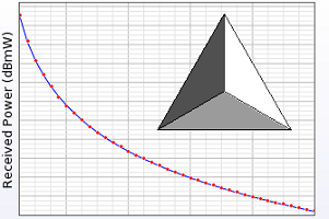
Double-click on the Received Power vs. targetLocation graph in the Project Tree to view the plot generated by the radar range equation script.

Verify that the plot generated by the radar range equation matches the simulated results.