Custom radiation patterns can be used in a project when data is written to *.uan files that are imported into WaveFarer. Once the antenna patterns are placed in WaveFarer, users can then complete the import verification steps that compose the second part of the project.
The first part of this tutorial examines a 77 GHz radar that was simulated in XFdtd, where 3D radiation patterns were determined for a transmitter and two receivers. That data is written to three *.uan files, which are then imported into WaveFarer as antenna definitions. A transceiver containing 1 transmitter with a 77 GHz waveform frequency and 2 receivers is created in order to locate the antennas at the origin.
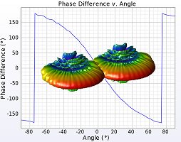
The second part of this tutorial includes creating a parameterized sphere and sweeping the simple scattering object across the front of the radar. A simulation is run with a parameter sweep from -90 to 90 degrees at 1 degree increments, and at each point along the arc, WaveFarer simulates the signal's scattering off of the sphere. Once the 180 degree sweep is complete, the phase difference between the two receivers compared against the expected results. The phase difference results confirm that the antenna patterns were imported correctly.
This tutorial utilizes the following skills:
- Importing *.uan files from an XF project as antenna definitions.
- Adding a transceiver consisting of one transmitter with a waveform frequency of 77 GHz and two receivers.
- Creating and applying both a distance and rotation parameter.
- Adding a sphere and sweeping its location by 180 degrees at a distance of 10 meters from the origin.
- Assigning a PEC material to the sphere in order to define the scattering target's electromagnetic properties.
- Setting the analysis configuration to include 1 reflection, 0 diffractions, and facet targeting.
- Writing and executing a script that animates the geometry and confirms correct parameter sweep behavior.
- Running a simulation that performs parameter sweep from -90 to 90 degrees at 1 degree increments.
- Evaluating the phase difference between the two receivers.
Step 1: Import the Antennas
Custom radiation patterns can be used by importing *.uan files. This tutorial requires three antenna definitions.
- Prepare three *.uan files.
- Right-click on Antennas in the Project Tree and select New Antenna Definition.
- Enter the New Antenna name by typing Tx into the highlighted field.
- Press Enter to apply the name change.
- Double-click on the antenna in the Project Tree to open the Antenna Editor.
- Use the Type drop-down arrow to select User-defined.
- Under the Properties tab, click Select UAN file to import.
- Choose the associated *.uan file.
- Click Open to load the imported file in the Antenna Editor.
- Click Done to close the editor.
- Repeat steps 2 – 10 to import the first receiver, using Rx 1 as the name.
- Repeat steps 2 – 10 to import the second receiver, using Rx 2 as the name.
Step 2: Add a Transceiver
The transceiver serves as the point where the rays are sent and received. For this tutorial, it will consist of one transmitter and two receivers with associated antenna and waveform definitions.
First, create the transceiver.
- Right-click on the Transceivers branch of the Project Tree and select New Transceiver Points Layout to open the editor.
- Under the Layout tab, click in the Type field and use the drop-down arrow to select Transmitter.
- Check the box in the next column to enable the Activates the antenna pattern for viewing at this location option.
- Click Zoom to Extents in the right sidebar, then zoom in using the middle mouse wheel.
- Check the Changes to Radius Affects All Points option.
- Click in the Radius column of and enter 1.5 mm.
- Click the
 button on the right side of the Layout tab to add the first receiver.
 - Click in the Type field and use the drop-down arrow to select Receiver.
- Click in the Antenna field and use the drop-down arrow to select Rx 1.
- Click the button on the right side of the Layout tab to add the second receiver.
- Click in the Antenna field and use the drop-down arrow to select Rx 2.
- Press Enter to apply the changes.
- Select the first point in the table by clicking on Transmitter.
- Toggle the orientation-editing settings by clicking the
 button at the top of the tab.
 - Enter -15 mm as the Y value.
- Press Enter to apply the change.
- Set the Point to 2 to edit the location of the first receiver.
- Enter 14 mm as the Y value.
- Press Enter to apply the change.
- Set the Point to 3 for the second receiver.
- Enter 16 mm as the Y value.
- Press Enter to apply the change.
- Name the transceiver by typing Transceiver w/ 1 Tx, 2 Rx into the Name field.
- Click Done to close the editor.
Then, set the waveform's properties.
- In the Definitions branch of the Project Tree, double-click on the Sinusoid waveform to open the Waveform Editor.
- Enter 77 GHz as the Frequency.
- Name the waveform by typing 77 GHz Sinusoid into the Name box.
- Click Done to close the editor.
Verify the change by opening the transceiver editor and checking the transmitter's property.
Step 3: Create a Parameterized Sphere
Once the antennas are defined, users can begin part two of the project, which verifies the import. The scattering object will be modeled as a sphere, and then translated and rotated by applying two parameters.
First, create the part.
- Right-click on the Parts branch of the Project Tree and select Create New ❯ Sphere.
- Enter 0.05 m as the Radius value.
- Click Done to close the editor.
Next, define the parameters.
- Click the Parameters button on the right-side of the WaveFarer window.
- Click the button.
- Type translationDistance into the Name field.
- Press Tab and enter 10 m in the Formula field.
- If desired, hit Tab and enter a brief description.
- Click the button.
- Type rotationAngle into the Name field.
- Press Tab and enter 90 deg in the Formula field.
- Click Apply and close the Parameters window.
Then, modify the geometry.
- Right-click on Sphere in the Parts branch of the Project Tree and select Modify ❯ Transform ❯ Translate.
- Under the Specify Translation tab, enter the translationDistance parameter as the U value.
- Click Done to close the editor.
- Right-click on Sphere in the Parts branch of the Project Tree and select Modify ❯ Transform ❯ Rotate.
- Under the Specify Rotation tab, enter the rotationAngle parameter as the Angle value.
- Click Done to close the editor.
Verify that the Sphere moves according to the parameter's Formula by changing the definition to 45 deg in the Parameters window, clicking Apply, and checking the bounding box in the Geometry window.
Step 4: Define and Assign a PEC Material
A material needs to be associated with the geometry in order to determine its scattering behavior, so a material first needs to be defined and then assigned to the sphere. WaveFarer's definitions node allows users to define a set of electromagnetic properties once and use that definition in multiple places, although this tutorial is basic and requires just one.
First, define the material.
- Right-click on Materials in the Project Tree and select New Material Definition.
- Enter the material name by typing PEC into the highlighted field.
- Press Enter to appply the name change.
- Double-click on the material to open the Material Editor.
- Change the Type to Perfect Electrical Conductor (PEC) using the drop-down arrow.
- If desired, navigate to the Appearance tab and choose the PEC material's display color.
- Click Done to finish the PEC material.
Then, assign the material to the Sphere.
- Click-and-drag the PEC material from the Definitions branch of the Project Tree and drop it on top of the Sphere in the Parts branch of the Project Tree.
Step 5: Set the Analysis Configuration
Users can enter inputs in the analysis configuration settings that control how the calculation engine evaluates the simulation space, modifying the tradeoff between accuracy and run time. The reflection and diffraction values determine the maximum amount of interactions a ray path can have with geometry faces and edges. Higher numbers increase accuracy, as well as run time.
- Right-click on Analysis Configurations in the Project Tree and select New Physical Optics Configuration.
- Enter the configuration name by typing 1R0D into the highlighted field.
- Press Enter to apply the name change.
- Double-click on the configuration in the Project Tree to open the Physical Optics Configuration Editor.
- Under the Properties tab, enter 1 as the Number of Reflections.
- Enter 0 as the Number of Diffractions.
Note that the remaining default settings are desired for this project. Confirm that Minimum Angular Ray Spacing is 0.01 degrees, Restrict Rays By Gain Threshold is checked with a value of 30 dBi, Include MEC Diffractions is checked, and Allow Knide Edges is unchecked.
- Click Done to close the editor.
Step 6: Animate the Scenario
Once the project is set up, users can animate the geometry by writing and executing a script. This step is not required, but it is recommended because it provides visual confirmation that the parameter sweep will behave as expected when the simulation is created.
- Right-click on the Scripts branch of the Project Tree and select New Macro Script to open the Scripting window.
- Right-click on New Macro Script in the Project Tree and select Rename.
- Enter the script's name by typing Sweep rotationAngle into the Project Tree.
- Press Enter to apply the name change.
- Enter the script in the Scripting window:
for( var a = -90; a <= 90; ++a )
{
list.setFormula( "rotationAngle", a + " deg" );
App.sleep( 20 );
}
- Save the script by clicking the commit icon in the toolbar.
Verify the script by right-clicking on Sweep rotationAngle in the Project Tree and selecting Execute to watch the Sphere rotate around the origin in the Geometry window.
Step 7: Create and Run a Simulation
Once the project is complete, it must be saved in order to create a new simulation and write output files.
First, save the project.
- Click File in the upper-left corner of the WaveFarer window, then select Save Project As.
- Enter User-Defined Antennas as the project name.
- Click Save.
Then, create and run the simulation.
- Click the Simulations button in the upper-right corner of WaveFarer to open the Simulations window.
- Click the Create New Simulation button in the upper-left corner of the Simulations window.
- In the Create Simulation window, enter the simulation name by typing Sweep -90 to 90 deg at 10 m into the Name box.
- Select 1R0D as the Configuration using the drop-down arrow.
- If applicable, change the Resource tab settings to match the hardware that will run the simulation.
- Under the Setup Parameter Sweep tab, check the Perform Parameter Sweep option.
- Click the
 button to define a parameter sweep.
 - Confirm that rotationAngle is the parameter to sweep.
- Use the Sweep Type drop-down arrow to select Start, End, Count.
- Enter 181 as the Count value.
- Enter -90 deg as the Starting Value.
- Enter 90 deg as the Ending Value.
Verify that the Evaluated Values are between -90 degrees and 90 degrees with 1 degree increments (i.e., -90 deg, -89 deg, -88 deg, etc.).
- Click Create & Queue Simulation.
Notice that the simulation now appears at the top of the Simulations window, and the Sweep field indicates which of the 181 parameter values are being simulated. The Status field will change to Complete when the simulation is finished and the results have been generated.
Step 8: Graph the Phase Difference
The simulation's results are available, and the received power at each receiver can be plotted against the project's defined parameter by running a script. A second macro will be used to plot the phase difference between the receivers. Both scripts must first be downloaded, and are available on the support site using the links found in the sidebar of this tutorial page.
First, generate a graph of received power.
- Download the Plot Received Power Versus Parameter script and save it in WaveFarer's macros folder.
- In the upper-left corner of WaveFarer, select Macros, then Results ❯ Plot Received Power Versus Parameter to open the editor.
Note that the Project, Simulation, and Sensor settings each have only one available option.
- Change the Complex Part by selecting Phase from the drop-down menu.
- Click OK to change the editor.
Note that the parameter's name appears between brackets, but the units associated with it were not stored with the simulation. Also, the three transceiver boxes checked by default will plot the received power for both Rx 0 and Rx 1 from Tx 0 versus distance, which is desired for this project.
- Change the parameter's units by selecting Angle from the drop-down menu.
- Click OK to change the editor a second time.
Note that an XY graph will be created and its title and labels can be customized.
- Click OK to close the editor.
Verify that the graph appears in the Graphs branch of the Project Tree and double-click on it to view.
Then, use a second script to plot the phase difference.
- In the upper-left corner of WaveFarer, select Macros, then Results ❯ Plot Phase Difference to open the editor.
Note that the upper portion of the editor specifies Rx 0 and Rx 1 as Plot A and Plot B, respectively. This indicates that the received power graph is the data source and we will compute the difference between its two plots.
- In the Destination portion of the editor, enter the Plot Name by typing Rx 0 - Rx 1.
- Click OK to close the editor.
Verify that the phase difference plot matches the expected results based on the XF project from step 1.