XF's Debye-Drude material definition offers two dispersive models—Debye and Drude—whose complex permittivity varies with frequency. The models support multiple poles for more flexibility when fitting the XF material to a set of measured data. Because XF uses the finite-difference time-domain (FDTD) method, a single simulation includes this dispersion over a range of frequencies, for example 850 MHz to 6 GHz.
Debye-Drude Material | XFdtd
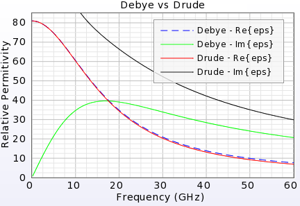
![]() Electric dispersive material definition.
Electric dispersive material definition.