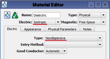
An electric nondispersive material's properties—$\epsilon_r$ and $\sigma$— do not vary with frequency. This material is defined by choosing Isotropic as the Electric setting at the top of the Material Editor and selecting Nondispersive from the Type drop-down menu. XF supports multiple nondispersive and dispersive entry methods, but they all conform to a linear, isotropic, nondispersive material expressed by Maxwell's equation
\begin{equation} \epsilon_r\epsilon_0\frac{\partial E (t)}{\partial t} = \nabla \times H(t) - \sigma E (t) \end{equation}where
$\epsilon_r = $ electric relative permittivity
$\epsilon_0 \simeq 8.85 \times 10^{-12} = $ free space permittivity (farads/meter)
$\sigma = $ electric conductivity (Siemens/meter)
For each Entry Method, the Good Conductor setting determines whether the material is considered a high-conductivity material for the purposes of PrOGrid regions and XACT meshing. The default Automatic setting classifies the material as a good conductor if it satisfies $\sigma \geq 1000 \omega\epsilon$ at the center of the project's frequency range of interest. The ON and OFF settings can each be used to override this automatic behavior.
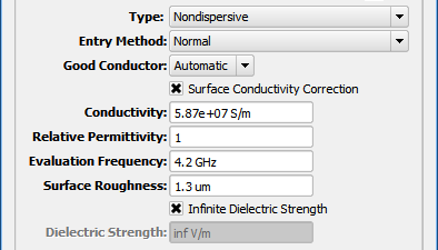
The Evaluation Frequency is used to convert a frequency-dependent equation into the nondispersive definition. Because the Evaluation Frequency accepts a single value, it should be set to the operating frequency of the device or the center frequency of the band in order to achieve the most accurate results. In order to simulate a material that varies over a wide band, it may be necessary to change the evaluation frequency and run multiple simulations.
The Infinite Dielectric Strength option applies to electrostatic discharge (ESD). In order to perform this analysis, users must uncheck the box and provide a finite dielectric strength value. This parameter does not factor into Maxwell's equations for computing electric and magnetic fields; it is only used to detect possible dielectric breakdown in ESD analysis.
Entry Methods
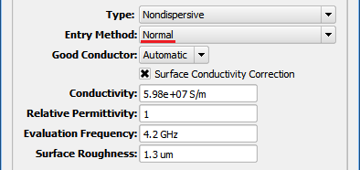
The Normal Entry Method allows both $\epsilon_r$ and $\sigma$ to be entered directly into the Relative Permittivity and Conductivity fields, respectively. Surface Conductivity Correction adjusts the conductivity value in order to preserve the desired surface impedance of the material. This setting should be checked for high-conductivity materials, like copper and other metals. Because surface impedance is frequency dependent, the Evaluation Frequency must be entered. Users can also enter a Surface Roughness value to account for the irregular surface where a copper trace is bonded to a substrate. Providing a surface roughness value is particularly important at frequencies above 3 GHz where the current flowing along a copper trace moves closer to the surface as the skin depth decreases.
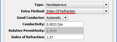
The Index of Refraction Entry Method allows $\sigma$ to be entered directly into the Conductivity field. Index of Refraction, $n$, must be entered in order to determine relative permittivity based on $n = \sqrt{\epsilon_r}$.
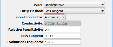
The Loss Tangent Entry Method allows $\epsilon_r$ to be entered directly into the Relative Permittivity field. Loss Tangent, $\text{tan }\delta$, and Evaluation Frequency, $f$, must be entered in order to determine conductivity based on $\text{tan }\delta = \sigma/2\pi f\epsilon_r\epsilon_0$.
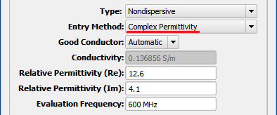
The Complex Permittivity Entry Method takes the form ${\epsilon_r}'-j{\epsilon_r}''$. ${\epsilon_r}' = \epsilon_r$ and is entered directly into the Relative Permittivity (Re) field, and $\sigma$ is determined by using Relative Permittivity (Im) and Evaluation Frequency, $f$, based on ${\epsilon_r}'' = \sigma/2\pi f\epsilon_0$.
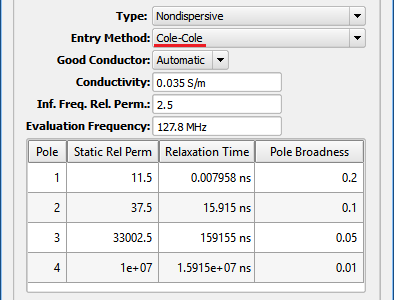
The Cole-Cole Entry Method is often used for biological tissue materials. It has four poles and takes the form
\begin{equation} \epsilon(\omega) = \epsilon_\infty + P_1 + P_2 + P_3 + P_4 + \frac{\sigma}{j\omega\epsilon_0} \end{equation}where
\begin{equation} P_n = \frac{\epsilon_{s,n}-\epsilon_\infty}{1+(j\omega t_{0,n})^{1-\alpha_n}}, \,\,\,\, n=1,2,3,4 \end{equation}and
- $\epsilon_\infty = $ relative permittivity at infinite frequency
- $\epsilon_{s,n} = $ static relative permittivity of pole n
- $\omega = $ radian frequency
- $t_{0,n} = $ relaxation time of pole n
- $\alpha_n = $ broadness of pole n
- $\sigma = $ conductivity