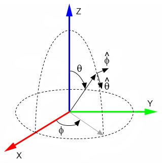
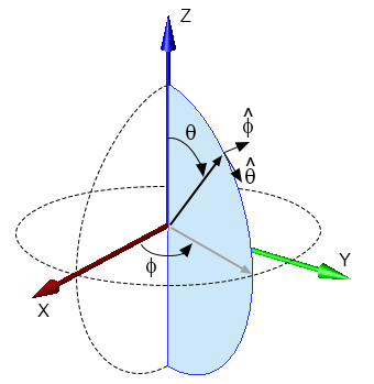
XF uses the theta, phi coordinate system's $\theta$ and $\phi$ values to define far zone observation points and a plane wave's incident direction. In the coordinate system, $\theta$ is defined as the angle between the positive z-axis and an observation point and has a typical range of 0 to 180 degrees. The $\phi$ angle is defined as being between the positive x-axis and the observation point projected onto the XY plane and its typical range is between 0 and 360 degrees.
Electromagnetic fields can be broken into $E_{\theta}$ and $E_{\phi}$ vector components at the observation point ($\theta$, $\phi$). $\hat{a_{\theta}}$ and $\hat{a_{\phi}}$ are the associated unit vectors.
\begin{equation} E(\theta,\phi) = E_{\theta}\hat{a_{\theta}} + E_{\phi}\hat{a_{\phi}} \end{equation}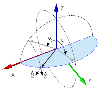
XF uses the alpha, epsilon Ludwig 2 coordinate system's $\alpha$ and $\epsilon$ values to define far zone observation points. In the coordinate system, $\alpha$ is defined as the angle between the positive z-axis and the observation point projected onto the XZ plane and has a typical range of -90 to 90 degrees. The $\epsilon$ angle is defined as being between the positive z-axis and the observation point projected onto the YZ plane and its typical range is between 0 and 360 degrees.
Electromagnetic fields can be broken into $E_{\alpha}$ and $E_{\epsilon}$ vector components at the observation point ($\alpha$, $\epsilon$). $\hat{a_{\alpha}}$ and $\hat{a_{\epsilon}}$ are the associated unit vectors.
\begin{equation} E(\alpha,\epsilon) = E_{\alpha}\hat{a_{\phi}} + E_{\epsilon}\hat{a_{\phi}} \end{equation}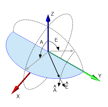
XF uses the elevation, azimuth Ludwig 2 coordinate system's $E$ and $A$ values to define far zone observation points. In the coordinate system, $E$ is defined as the angle between the positive z-axis and the observation point projected onto the YZ plane and has a typical range of -90 to 90 degrees. The $A$ angle is defined as being between the positive z-axis and the observation point projected onto the XZ plane and its typical range is between 0 and 360 degrees.
Electromagnetic fields can be broken into $E_{E}$ and $E_{A}$ vector components at the observation point ($E$,$A$). $\hat{a_{E}}$ and $\hat{a_{A}}$ are the associated unit vectors.
\begin{equation} E(E,A) = E_{E}\hat{a_{E}} + E_{A}\hat{a_{A}} \end{equation}Transform Observation Angles
The following equations transform an observation angle directly from one coordinate system to another.
($\theta$,$\phi$) from ($E$,$A$)
\begin{equation} \theta = \cos^{-1} (cos(E) cos(A)) \end{equation} \begin{equation} \phi = \tan^{-1} \biggl(\frac{sin(E)}{sin(A)cos(E)}\biggr) \end{equation}($E$,$A$) from ($\theta$,$\phi$)
\begin{equation} E = \sin^{-1} (sin(\theta) sin(\phi)) \end{equation} \begin{equation} A = \tan^{-1} \biggl(\frac{sin(\theta) cos(\phi)}{cos(\theta)}\biggr) \end{equation}($\theta$,$\phi$) from ($\alpha$,$\epsilon$)
\begin{equation} \theta = \cos^{-1} (cos(\alpha) cos(\epsilon)) \end{equation} \begin{equation} \phi = \tan^{-1} \biggl(\frac{cos(\alpha) sin(\epsilon)}{sin(\alpha)}\biggr) \end{equation}($\alpha$,$\epsilon$) from ($\theta$,$\phi$)
\begin{equation} \alpha = \sin^{-1} (sin(\theta) cos(\phi)) \end{equation} \begin{equation} \epsilon = \tan^{-1} \biggl(\frac{sin(\theta) sin(\phi)}{cos(\theta)}\biggr) \end{equation}Transform Vector Components
Vector components are transformed indirectly from one coordinate system to another. First, they must be transformed into the intermediate cartesian coordinate system using the following equations.
$E_{\theta}$ and $E_{\phi}$ vector components to $E_x$, $E_y$, and $E_z$
\begin{equation} \begin{bmatrix} E_{x}\\ E_{y}\\ E_{z}\\ \end{bmatrix} = \begin{bmatrix} E_{\theta}cos(\phi)cos(\theta)-E_{\phi}sin(\phi)\\ E_{\theta}sin(\phi)cos(\theta)+E_{\phi}cos(\phi)\\ -E_{\theta}sin(\theta) \\ \end{bmatrix} \end{equation}$E_{\alpha}$ and $E_{\epsilon}$ vector components to $E_x$, $E_y$, and $E_z$
\begin{equation} \begin{bmatrix} E_{x}\\ E_{y}\\ E_{z}\\ \end{bmatrix} = \begin{bmatrix} E_{\alpha}cos(\alpha)\\ -E_{\alpha}sin(\epsilon)sin(\alpha)+E_{\epsilon}cos(\epsilon)\\ -E_{\alpha}cos(\epsilon)sin(\alpha)-E_{\epsilon}sin(\epsilon) \\ \end{bmatrix} \end{equation}$E_{E}$ and $E_{A}$ vector components to $E_x$, $E_y$, and $E_z$
\begin{equation} \begin{bmatrix} E_{x}\\ E_{y}\\ E_{z}\\ \end{bmatrix} = \begin{bmatrix} -E_{E}sin(E)sin(A)+E_{A}cos(A)\\ -E_{E}cos(E)\\ -E_{E}cos(A)sin(E)-E_{A}sin(A) \\ \end{bmatrix} \end{equation}Vector components in the cartesian coordinate system can then be transformed into the final coordinate system using the following equations.
$E_{\theta}$ and $E_{\phi}$ vector components from $E_x$, $E_y$, and $E_z$
\begin{equation} \begin{bmatrix} E_{\theta}\\ E_{\phi}\\ \end{bmatrix} = \begin{bmatrix} E_{x}\, cos(\phi)cos(\theta)+E_{y}\, sin(\phi)cos(\theta)-E_{z}\, sin(\theta)\\ -E_{x}\, sin(\phi)+E_{y}\, cos(\phi)\\ \end{bmatrix} \end{equation}$E_{\alpha}$ and $E_{\epsilon}$ vector components from $E_x$, $E_y$, and $E_z$
\begin{equation} \begin{bmatrix} E_{\alpha}\\ E_{\epsilon}\\ \end{bmatrix} = \begin{bmatrix} E_{x}\, cos(\alpha)-E_{y}\, sin(\epsilon)sin(\alpha)-E_{z}\, cos(\epsilon)sin(\alpha)\\ E_{y}\, cos(\epsilon)-E_{z}\, sin(\epsilon)\\ \end{bmatrix} \end{equation}$E_{E}$ and $E_{A}$ vector components from $E_x$, $E_y$, and $E_z$
\begin{equation} \begin{bmatrix} E_{E}\\ E_{A}\\ \end{bmatrix} = \begin{bmatrix} -E_{x}\, sin(E)sin(A)-E_{y}\, cos(E)-E_{z}\, sin(E)cos(A)\\ E_{x}\, cos(A)-E_{z}\, sin(A)\\ \end{bmatrix} \end{equation}