Compute Average Power Density – XFdtd

XFdtd's algorithm for computing spatial-average power density (sPD) and peak spatial-average power density (psPD) adheres to the international standard IEC/IEEE 63195-2 [1].

Prerequisites

IEC/IEEE 63195-2 provides an algorithm for testing emissions from a radiating device. In addition to setting up an XF project to simulate a radiating device, an evaluation surface must be provided where power density is calculated.

Often, the evaluation surface must be a specific distance from the device at a location that does not coincide with a gridline. The user must therefore specify a planar or non-planar sensor in order to define the evaluation surface, as well as a volume sensor that surrounds the evaluation surface. The script then interpolates the fields of the volume sensor onto the evaluation surface.

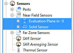
Create a Planar Sensor, Rectangular Sensor, or Sensor on Model Surface to serve as the evaluation surface.
Collect steady-state electric fields in the associated Surface Sensor Definition.
Create a Solid Box Sensor that is larger than the planar sensor, surrounding it by one cell edge in all directions.
Collect steady-state electric and magnetic fields in the associated Solid Sensor Definition.
Specify one or more steady-state frequencies when creating the FDTD simulation.
Run the FDTD simulation to completion.

Multiple evaluation surfaces could potentially be surrounded with a single, large solid sensor.

Workflow

After meeting the prerequisites, run the macro by following these steps:

Download the Compute Average Power Density.xmacro
Right-click on Scripts in the Project Tree and select Import Scripts.

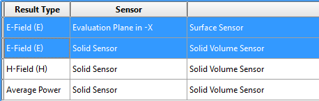
Once the script is available, select two result sensors for analysis.

Open the Results browser.
Specify the evaluation surface by left-clicking on a planar or non-planar sensor result in the lower portion of the Results browser.
Press Shift while left-clicking on a volume sensor result in the lower portion of the Results browser in order to specify the associated electric fields.
Double-click on Compute Averaged Power Density in the Scripts branch of the Project Tree to open the Scripting window.
Click Execute at the top of the window, then select Execute Macro to open the Average Power Density window.

Selecting the magnetic fields is unnecessary because the script accesses them based on the name of the selected solid sensor.

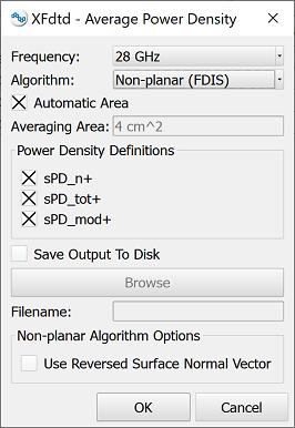
Specify the calculation inputs.

Use the Frequency drop-down arrow to choose from the list of steady-state frequencies specified when creating the FDTD simulation.
Use the Algorithm drop-down arrow to choose from the list of algorithms.

Verify that the Automatic Area option is selected by default in order to set the averaging area size based on the frequency. The averaging area is a square that is 4 cm² for frequencies less than or equal to 30 GHz, and 1 cm² for frequencies greater than 30 GHz. Unchecking this option requires users to enter a custom size into the associated field.

The standard includes three equations for computing sPD:

Section 8.5.2 Surface-normal propagation-direction power density into the evaluation surface - sPD_n+
Section 8.5.3 Total propagating power density into the evaluation surface - sPD_tot+
Section 8.5.4 Total power density directed into the phantom considering near field exposure - sPD_mod+

Specify one or more sPD equations to use.

In the Power Density Definitions section, select sPD_n+ to use the equation in Section 8.5.2., sPD_tot+ to use the equation in Section 8.5.3., and sPD_mod+ to use the equation in Section 8.5.4.

Visualize sPD data on the evaluation surface in Matlab.

If desired, select the Save Output to Disk option to save sPD at each vertex on the evaluation plane to a Matlab *.m file.
If the Save Output to Disk option is selected, either specify the output file and location by clicking the Browse button, or enter the file into the Filename field.

If the non-planar algorithm is selected, XF cannot guarantee that the normal of the evaluation surface is pointed into the phantom.

Select the Use Reversed Surface Normal Vector option to flip the direction of the evaluation surface normal.
Click OK.

The script triangulates the evaluation surface and computes sPD for each vertex using the electric and magnetic field data from the solid sensor. The psPD appears in a dialog window once the script is complete. If specified, the sPD is written to an output file.

Reference

International Electrotechnical Commission (IEC) and the Institute of Electrical and Electronics Engineers (IEEE), IEC/IEEE 63195-2, Assessment of Power Density of Human Exposure to Radio Frequency Fields from Wireless Devices in Close Proximity to the Head and Body (Frequency Range of 6 GHz to 300 GHz) - Part 2: Computational Procedure, 2022.