Modal Waveguide Excitation | XFdtd

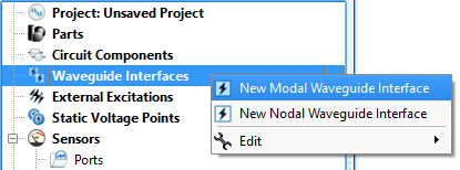
Open the modal waveguide editor by right-clicking on Waveguide Interfaces in the Project Tree and selecting New Modal Waveguide Interface.

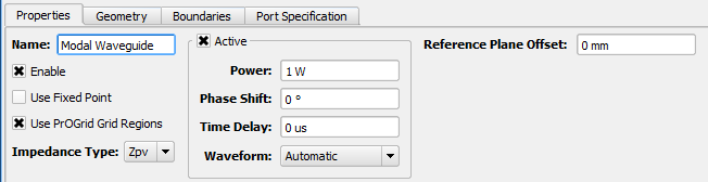
Under the Properties tab, basic attributes can be defined:

• Name: a user-defined descriptor that will be referenced when creating simulations and analyzing results.
• Enable: includes the waveguide interface in the simulation. Unchecking Enable effectively removes an interface from a project without deleting it, so it is available for use later.
• Use Fixed Point: adds a fixed point to the grid in the plane of the interface.
• Use PrOGrid Grid Regions: includes the interface in the PrOGrid formulation which adds boundary refinements to each of the four edges that make up the rectangle of the waveguide interface. These refinements reduce cell sizes near the waveguide interface in both the propagation direction and the transverse directions. Boundary refinements for waveguides are consistent with the main grid editor’s good conductor boundary refinement ratio and boundary refinement number of cells settings.
• Impedance Type: type of impedance computation, Z_vi, Z_pv, Z_pi.
• Active: allows a mode to be excited. Uncheck Active to use this waveguide interface as a matched termination only.
• Power: peak instantaneous power available to the waveguide. When computing S-parameters, 1 W power is used.
• Phase Shift: phase shift applied to the associated waveform, but only if the waveform is a sinusoid.
• Time Delay: applied to the associated waveform, but only if the waveform is not a sinusoid.
• Waveform: associated waveform definition. The selected waveform will be applied to active modes.
• Reference Plane Offset: a positive value moves the reference plane for the S-parameters computation along the waveguide's propagation direction. This is useful in cases where it is inconvenient to position the interface plane at the precise location where S-parameters should be computed. Users should note that this assumes there is no change in waveguide propagation characteristics between the interface plane and reference plane, such as would occur due to a change in waveguide cross sectional geometry.

Users should note that either Phase Shift or Time Delay will be applied depending on whether or not the waveform is sinusoid.

XF has three options for calculating impedance:

\begin{equation} Z_{pv}(f)=\frac{V(f)V^*(f)}{2P(f)} \end{equation} \begin{equation} Z_{vi}(f)=\frac{V(f)}{I(f)} \end{equation} \begin{equation} Z_{pi}(f)=\frac{2P(f)}{I(f)I^*(f)} \end{equation}

where $P(f)$, $V(f)$, and $I(f)$ are complex frequency-domain power, voltage, and current, respectively, and $A^*$ indicates the complex conjugate of $A$. To extend these definitions to waveguides, let $P(f)\rightarrow P_t(f)$ be the power flow through the transverse cross section of the guide and $I(f)$ be the total current flow. $P_t(f)$ and $I(f)$ are thus well defined. The usual way to obtain voltage, $V(f)$, is to integrate the electric field along an integration line in the transverse plane of the waveguide between terminals or sides of the guide. The integration line, discussed later, defines this path for the computation of $V(f)$ and must be defined to compute $Z_{pv}$ or $Z_{vi}$. Users should note that in circuit theory, $Z_{pv}=Z_{vi}=Z_{pi}$. Because $V(f)$ is path-dependent, $Z_{pv}\neq Z_{vi}\neq Z_{pi}$ in general waveguide theory.

The Geometry tab provides tools for specifying the location, size, and propagation direction of the interface. The Boundaries tab is used to specify the behavior of the four interface edges.

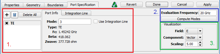
Under the Port Specification tab, there are three groups of controls:

1. Port specification.
2. Field computation.
3. Field visualization.

Here, modes and ports are equivalent and interchangeable. Ports are used in the user interface to be consistent with circuit theory, where ports excite the space and S-parameters are computed between them. Add and delete ports using the and buttons, respectively. A port that is checked will be part of a simulation and may be set as the active port when a simulation is created. If there are no ports, it will act as a matched termination.

One port in the ports list will appear in bold text, indicating that it is the default port and will be active if S-parameters are not computed. Right-click on a port and select Make Default to change it to the default port.

Port information—such as line impedance, wave impedance, and beta—is provided in the Port Info tab once modes are computed.

• Type: Type can be TE for transverse electric, TM for transverse magnetic, TEM for transverse electric and magnetic, quasi-TEM for quasi-transverse electric and magnetic, such as a microstrip, or EH for mixed modes having both TE and TM components.
• Fc: Cutoff frequency, $f_c$, of lowest propagating frequency of the chosen mode.
• Beta: Propagation constant, $\beta$, of the chosen mode in the waveguide.
• Zwave: Wave impedance, $Z_w$, is the ratio of the transverse components of the electric and magnetic fields in the waveguide. It is computed by $\sum_{cells}\frac{|E_t(f)|}{|H_t(f)|}$ in the plane of the port, where $E_t(f)$ and $H_t(f)$ are the transverse components of $E$ and $H$, respectively, and $f$ is the evaluation frequency.
• Zline: Line impedance, $Z_l$, is computed when XF detects a transmission line, meaning two or more unattached conductors. Examples include a microstrip, stripline, coax, and differential pair. It is computed by $\frac{P_t(f)}{I^2(f)}$, where $P_t(f)$ is the frequency-domain forward power and $I(f)$ is the frequency-domain forward current for the port.

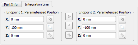
The Integration Line is used to compute voltage and orient modes when there is rotational symmetry. It can be specified for each mode before or after clicking Compute Modes by checking Use Integration Line. This enables the Integration Line tab, where the values can be defined using the picker tools. The positive zero-phase direction will be set so that the electric fields point from Endpoint 2 toward Endpoint 1.

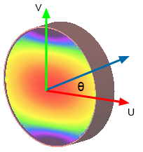
In certain cases where the waveguide cross section contains rotational symmetry, such as in a square or circular waveguide, it may be possible for a mode to exist in more than one orientation. For example, if the desired orientation angle in a circular waveguide is defined as θ for the mode relative to the positive direction of the u-axis, then θ can vary from 0 to 2π without changing mode type, $\beta$, $f_c$, or $Z_w$ for the mode. This ambiguity is a type of mode degeneracy, so XF will orient the mode so that the strongest electric field is parallel to the u-axis. If another orientation is desired, the integration line can be used to orient the mode within the waveguide. The direction of the line—endpoint 1 versus endpoint 2—determines the positive direction of the fields, so it is important to define integration lines consistently for like modes when S-parameters are being computed.

The evaluation frequency sets the frequency at which the modes are computed. This frequency needs to be higher than the cutoff frequency of modes defined for each of the ports. If it is set too low, a mode may not be found. The Evaluation Frequency should be set as close as possible to the center of the frequency range over which the user is interested in waveguide port results. Once a value is entered, click Compute Modes in order to generate the Port Info data and allow field visualization. When modes are computed, an eigensolver finds each mode by assuming that the waveguide cross section is part of an infinitely long structure of that cross section.

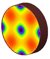
The Visualization settings render the modal field distributions in the geometry window for the selected port(s).

Simulate

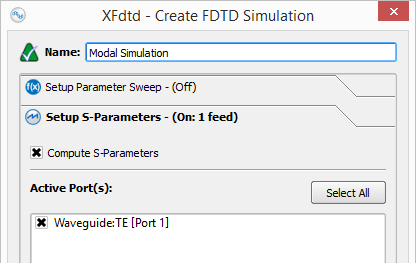
Set up a simulation either with or without S-parameters when modal waveguides are exciting the space. When S-parameters are enabled and more than one port selected, the simulation will contain one run for each selected port, where that port is active, and all other sources are inactive.

When S-parameters are disabled, the default port of the waveguide will be active with the power specified in the waveguide editor. The default port can be identified by expanding a waveguide interface in the Project Tree and finding the port in bold text and appended with Default Port. The default port can be changed by right-clicking on any of the ports and choosing Make Default.