 Far Zone Reference Settings allow users to set the reference point for computing radiated fields. This analysis is used when the phase difference between antenna elements requires careful design, such as an antenna array or radar.
Background
XF performs a surface integral over the fields near the boundary of the finite-difference time-domain (FDTD) space and it applies a near to far field transform in order to arrive at the radiated fields. This is an application of the surface equivalence theorem and the surface integral requires a reference point.
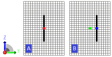
Consider the two projects in the first image. Project A has a half-wave dipole centered in the FDTD simulation space, and project B has a half-wave dipole offset λ/8 from the center. A 2-D far zone sensor is defined around the azimuth (XY) plane of the dipole in both projects and three simulations are run:
- Project A is simulated with the reference point set to the center of the space (co-located with dipole A).
- Project B is simulated with the reference point set to the center of the space (λ/8 offset from dipole B).
- Project B is simulated again with the reference point offset from the center of the space by λ/8 (co-located with dipole B).
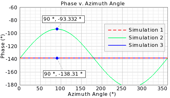
The second image shows the far zone phase for each simulation. When the reference point is co-located with the dipole, a constant phase is computed, but when the reference point is offset λ/8, the phase has a difference of 45° (138.3° - 93.3° = 45°) at 90° (along the y-axis). At 0° (along the x-axis) there is no difference in the far field phases.
Controls
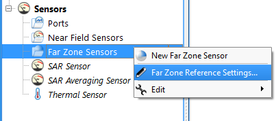
The Far Zone Reference Settings are accessed by right-clicking on the Far Zone Sensors item in the Project Tree. The settings consist of an editor across the top of the Geometry window where users can select a Mode option, which applies to all of the Far Zone Sensors in the project.
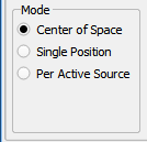 Center of Space is XF's default setting that determines the reference point based on the bounding box of the grid. This location may change between simulations if the the grid's size changes due to parameterized geometry or other settings.
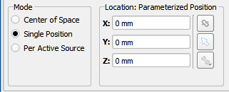 Single Position specifies a constant location for use as the reference point. Users can type values in the X, Y, Z boxes or use the three picker tool icons to the right in order to select a point based on geometry.
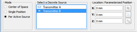 Per Active Source sets a unique phase reference point per feed when there are multiple feeds in a project. When using this mode, XF expects only one active feed per Simulation : Run—as is the case when S-parameters are requested.
Reference Point Post-Processing
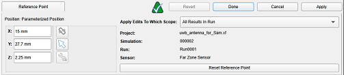
With reference point post-processing, users can dynamically adjust the reference point of far zone results without the need to adjust the Far Zone Reference Settings and perform additional simulations. The reference point determines the origin used for phase calculations in far field results.
Accessing the Reference Point Editor
Right-clicking on any steady state far zone entry in the results workspace window will show an option in the context menu to "Postprocess Far Zone Reference Point." This opens an editor that allows you to adjust the far zone reference point used for computing the result.
Scope Options
On the right-hand side of the editor there's a drop-down list where you can specify the range of results to adjust the reference point of:
- Current Result Only: Select this option to only change the reference point of the result that you had initially selected in the result browser.
- All Results In Run: Select this option to change the reference point of all far zone results in the selected result's run.
- Current Sensor For Entire Simulation: Select this option to change the reference point of all results for the selected sensor across all runs in the selected simulation.
- All Sensors In Simulation: Select this option to change the reference point of all far zone results in the selected simulation.
Important: The post-processed reference points are saved in the project and do not adjust the simulation data files. This feature modifies visualization and analysis only.
Phase Difference Plotting
By post-processing the reference point users can adjust the phase of a far zone result. To view the phase difference between two results, select two steady-state far zone results in the results workspace window and select the "Create Phase Difference Plot…" option in the context menu.
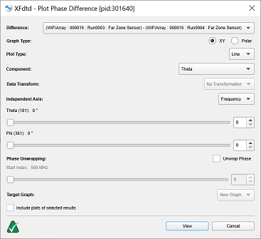
The Plot Phase Difference dialog is similar to the one used when creating plots for other results, but with a few extra options specific to phase differences:
- Difference: Select which order to perform the subtraction operation in. By default the phase of the second selected result will be subtracted from the phase of the first selected result.
- Phase Unwrapping: Click on the Unwrap Phase checkbox to enable phase unwrapping to get the results as a continuous line without discontinuities from angles wrapping around. Adjust the start index slider to pick the index on the independent axis that unwrapping will start from.
Understanding Phase Unwrapping
Phase unwrapping is necessary because phase angles are typically represented in the range of -180° to +180° (or 0° to 360°). When the actual phase exceeds these bounds, it "wraps around," creating discontinuities in the plot. Unwrapping removes these artificial jumps to show the true continuous phase progression.
Choosing the Start Index: The start index determines where the unwrapping algorithm begins. For best results, choose a start index in a region where the phase is smoothly varying and away from measurement noise or rapid phase changes.
Best Practices
- Use a common reference point when comparing multiple antennas or configurations to ensure meaningful phase comparisons.
- Apply reference point adjustments to all sensors in a simulation when performing system-level analysis.
- Save your project after adjusting reference points to preserve your post-processing settings.
- When creating phase difference plots, consider whether phase unwrapping is appropriate for your analysis—unwrapped phases show cumulative phase change, while wrapped phases emphasize periodic behavior.