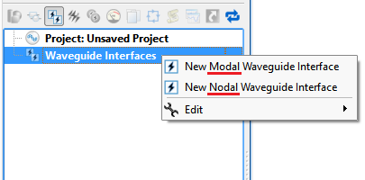
XF offers two waveguide interfaces—modal and nodal—for exciting a broad range of waveguide structures and transmission lines, including the classic rectangular or circular conducting pipes, microstrips, striplines, differential transmission lines, and coplanar waveguides. There is overlapping, and sometimes identical behavior between their excitations and results, but the nodal waveguide interface provides the unique ability to identify transmission line pins, specify a reference impedance, and compute renormalized S-parameters that exhibit an impedance mismatch at the source.
The following table shows which excitation is generally appropriate for the waveguide structure being analyzed:
| Modal | Nodal | |
|---|---|---|
| Classic Rectangular Waveguide | X | |
| Classic Circular Waveguide | X | |
| Coax | X | |
| Microstrip or Stripline | X | |
| Differential Microstrip or Stripline | X |
Concepts
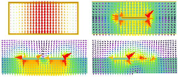
XF uses a 2-D eigensolver to find eigensolutions for the meshed geometry that exists in the cross section of the waveguide interface. Each eigensolution is referred to as a mode and takes the form of a TE, TM, TEM, or quasi-TEM field distribution. The modal waveguide interface uses these modes directly to excite the simulation space while the nodal waveguide interface uses a linear combination of the modes as an excitation. Users should note that the nodal and modal waveguide interface excitations are equivalent when there is only one signal conductor.
A modal excitation applies the eigensolution's field distribution directly to the waveguide structure or transmission line that is being fed. As such, the modal excitation is a matched excitation where the characteristic impedance of the waveguide interface is the same as that of the structure. A modal result implies that a mode excited the simulation space and there was no reflection at the interface due to an impedance mismatch.
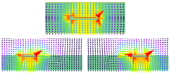
With a nodal excitation, a TEM or quasi-TEM single-ended field distribution is generated for each user-specified pin in a transmission line. These single-ended field distributions are generated based on a linear combination of the eigensolutions. For simulations that do not collect S-parameters, the single-ended field distribution is used to excite the space. A nodal result implies that one or more single-ended field distributions excited the space and there was no reflection at the interface due to an impedance mismatch. When S-parameters are collected, XF excites the space with the modal excitations then uses a modal to nodal conversion to compute the single-ended renormalized S-parameter matrix. The modal to nodal conversion includes a user-defined reference impedance resulting in a mismatch at the interface.
Users should note that the two nodal differential pair excitations are a linear combination of the odd and even modes above.
Workflow Comparison
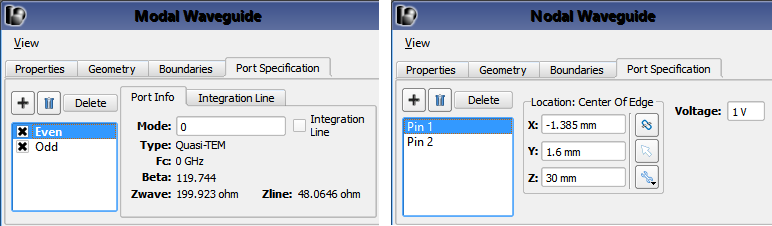
During the setup process, the properties, geometry, and boundaries tabs have equivalent meanings for modal and nodal waveguide interfaces. The difference between the modal and nodal waveguide arises in the port specification tab. For a modal waveguide interface, modes and integration lines are defined. These modes are determined by the eigensolver and there can be as many modes as the structure supports. For a nodal waveguide, pins are identified and single-ended field distributions are applied to each. The number of pins should be equal to the number of signal conductors at the interface.
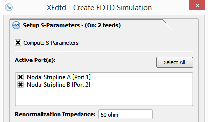
Creating a simulation is also a similar process for the two excitations. When S-parameters are enabled, users check which modes or pins should be excited for modal or nodal waveguide interfaces, respectively. Any combination of modes can be selected, but simulations with nodal waveguides require all pins to be selected. Additionally, entering the reference impedance is required for nodal waveguide interfaces in order to compute renormalize S-parameters.
In the results browser, results for waveguide interfaces are categorized into one of the sensor types—waveguide, waveguide mode, waveguide node, and renormalized S-parameters—corresponding to the terms outlined in the Concepts section above. The waveguide mode type is available for modal waveguide interfaces. Because a modal to nodal conversion is performed to compute renormalized S-parameters, waveguide mode and renormalized S-parameters are available for nodal waveguide interfaces when S-parameters are requested. When S-parameters are not requested for a nodal waveguide interface, the waveguide node type is available.
Stripline Example
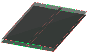
Consider a 20 ohm stripline that is 30 mm long with a pair of waveguide interfaces placed at either end. Two sets of simulations are run—one with modal waveguide interfaces and one with nodal waveguide interfaces—and impedance and S-parameter results are compared.
The stripline is a simple structure that supports only one TEM mode. As such, the modal and nodal excitations apply the same matched TEM field distribution to the transmission line. For each nodal waveguide interface, one pin is specified and the reference impedance is set to 50 ohms.
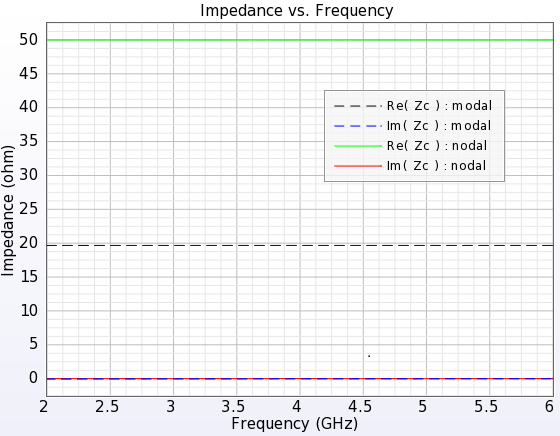
Both the modal and nodal waveguide interfaces produce modal results that show an impedance near 20 ohms. The nodal waveguide interface provides the user-specified characteristic impedance of the pin, which is 50 ohms.
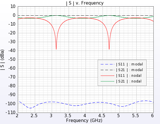
Both interfaces also produce modal S-parameter results that show no reflection at either end of the stripline. Renormalized S-parameters for the pins, however, show the mismatch due to the 50 ohm reference impedance.
In summary, both waveguide interfaces apply the same modal TEM excitation and produce modal results. The nodal waveguide interface provides the additional capability of identifying the pins and specifying a reference impedance for computing renormalized S-parameters.