The Waveform Editor defines waveforms used in conjunction with an excitation–circuit component, modal waveguide, nodal waveguide, or plane wave–in order to inject energy into the FDTD simulation space. The time-domain waveform is applied directly at each timestep during the finite-difference time-domain (FDTD) simulation. The frequency-domain content derived from the time-domain signal is also present and should be considered when choosing the time-domain signal.
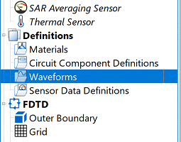
Users can access the Waveform Editor by right-clicking on Waveforms in the Definitions branch of the Project Tree, and selecting New Waveform Definition. A highlighted field appears in the Project Tree, allowing users to edit the assigned name before pressing Enter to add the waveform to the project.
Double-clicking on the waveform in the Project Tree opens the Waveform Editor, where the assigned name appears in the Name field. The Type drop-down menu lists the waveform options, each with specific settings appearing below once a selection is made.
The appropriate waveform type is determined by the desired analysis. For example, the broadband, and Gaussian-type waveforms are best for broadband calculations because they inject energy into the space in a wide band of frequencies.
Five buttons appear across the bottom of the editor:
- Revert: discards changes and restores the editor's settings to the previous saved version.
- Done: saves the entered specifications and closes the editor.
- Cancel: discards the entered specifications and closes the editor.
- Apply: saves the entered specifications and leaves the editor open.
Automatic
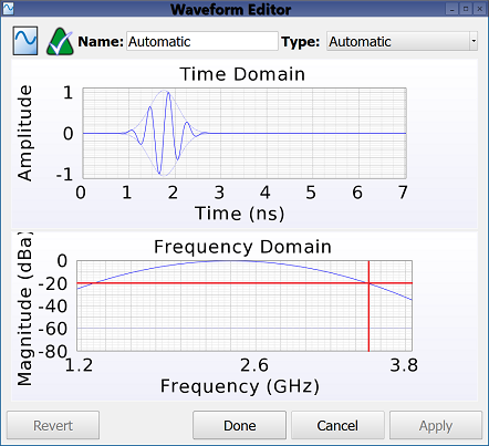
The default Automatic waveform changes shape in order to excite the project's frequency range of interest, and is recommended unless a specific time or frequency response is desired.
For a frequency range including 0 Hz, the waveform takes the shape of a Gaussian pulse that includes a DC component. For a frequency range excluding 0 Hz, the waveform takes the shape of a modulated Gaussian. In each of these broadband cases, the time-domain waveform is selected such that its frequency-domain content crosses -20 dB at the project's upper frequency of interest in order to avoid exciting frequencies outside the specified range.
For a project frequency range consisting of a single value, the waveform takes the shape of a sinusoid at the specified frequency. The automatic waveform adjusts to changes made to the project's frequency range of interest.
Gaussian
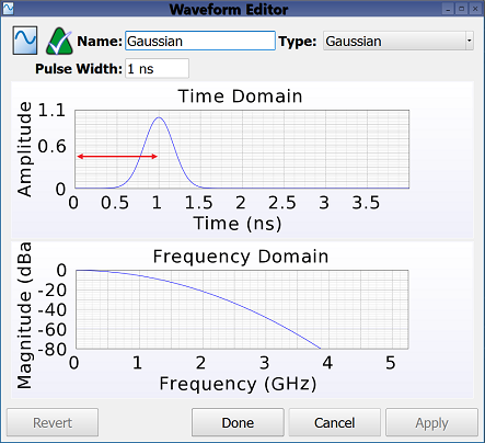
The Gaussian waveform shape is defined by the Gaussian function and contains a user-specified pulse width, $\eta$, attribute in seconds. The Gaussian pulse has a non-zero average value that produces a normal distribution on a conventional time-domain plot, with its bell-shaped curve centered around the pulse width. This waveform provides broadband input and is also suitable when broadband results are desired.
The Gaussian waveform is expressed by the following equation:
\begin{equation} f(t) = e^{-(t - \eta)^2 / 2\sigma^2} \end{equation}where $\sigma = \eta/\sqrt{32}$ is the standard deviation.
The Gaussian waveform is not recommended for use with a feed connected to a closed path unless the feed also contains resistance. This is because the Gaussian has a DC, or zero-frequency, component that starts a steady current flowing in a loop without decaying through loss or radiation, producing a source current with a non-zero average. In such cases, users could either specify a non-zero source resistence for the feed or choose one of the other two Gaussian waveforms.
Broadband
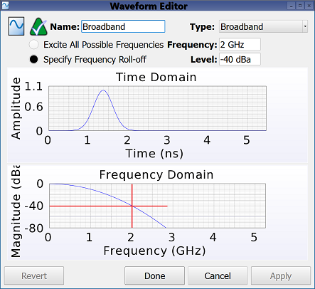
The Broadband waveform provides user-defined settings to specify a Gaussian pulse based on it's frequency-domain content.
This waveform has two options for defining a range of frequencies:
- Excite All Possible Frequencies: generates a time-domain waveform that produces the widest possible frequency content supported by the grid.
- Specify Frequency Roll-Off: generates a time-domain waveform with frequency-domain content matching the target specifications.
Selecting the Specify Frequency Roll-Off option enables two settings:
- Frequency: the target frequency specification.
- Level: the target magnitude specification.
Gaussian Derivative
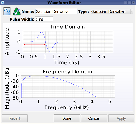
The Gaussian Derivative waveform is similar to the Gaussian insofar as it is defined by the Gaussian function and contains a user-specified pulse width, $\eta$, attribute in seconds. Unlike the Gaussian, this waveform's zero average produces a split-pulse shape that extends from a positive to negative amplitude. This waveform also does not include a DC component.
The Gaussian derivative waveform is expressed by the following equation:
\begin{equation} f(t) = \frac{t-\eta} {\sigma} e^{1/2 - (t - \eta)^2 / 2\sigma^2} \end{equation}where $\sigma = \eta/\sqrt{32}$ is the standard deviation.
Modulated Gaussian
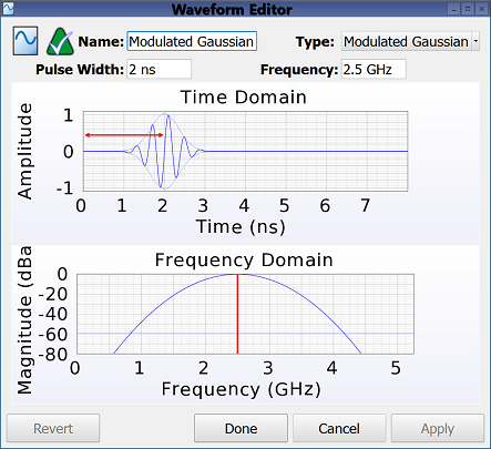
The Modulated Gaussian waveform is similar to both the Gaussian and Gaussian derivative insofar as it is defined by the Gaussian envelope and contains a user-specified pulse width attribute in seconds. Unlike the Gaussian, it includes a sinusoid at the specified Frequency and should therefore be used only when a specific frequency range is desired. The sinusoid is centered in the envelope so it has a zero-average pulse and does not include a DC component.
The modulated Gaussian waveform is expressed by the following equation:
\begin{equation} f(t) = Ne^{-(t - \eta)^2 / 2\sigma^2} \sin(\omega (t-\eta)) \end{equation}where $\sigma = \eta/\sqrt{32}$ is the standard deviation, $\omega$ is the angular frequency of the sinusoid, and $N$ is the normalization factor computed such that $f(t)$ has the maximum value of unity.
Adjusting the pulse width in order to enclose a specific frequency range is useful for exciting only frequencies in the band of single-mode operation, as well as simulating band-limited devices. For example, exciting a broadband antenna, such as a spiral, outside of the specific frequency range for which is designed, could greatly increase the simulation time needed for convergence. This is because the out-of-band energy cannot readily radiate or be otherwise dissipated by the antenna structure.
Sinusoid
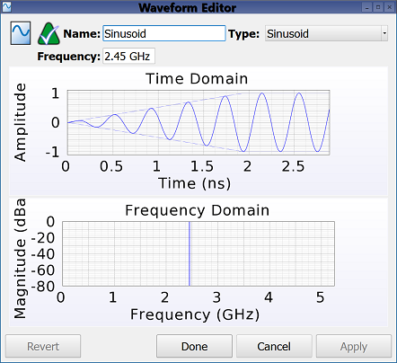
A Sinusoid waveform is useful when only one frequency is of interest. The ramped portion of the waveform is configured to avoid introducing energy into the simulation at any frequency other than that of the sinusoid.
A sinusoid waveform is expressed by the following equation:
\begin{equation} f(t) = (1-g(t)) \sin(\omega t + \phi) \end{equation}where $g(t)$ is a linear ramp based on the Bartlett window, and $\omega$ and $\phi$ are the angular frequency and phase of the sinusoid, respectively. Rather than setting $\phi$ through the waveform editor, a phase shift is applied through a feed definition, modal waveguide, or nodal waveguide.
User Defined
The User Defined waveform allows users to specify an arbitrary waveform by either importing a file or defining an equation. Users should refer to the user defined waveform documentation for an explanation of the controls, example equations, and the supported file format.