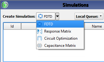
Once a completed project is saved, users can run calculations through the Simulations window by choosing FDTD as the Create Simulation option in the upper-left corner. In the Create FDTD Simulation window that opens, users can set up electromagnetic calculations to run through XF's calculation engine.
The Name field at the top of the window provides space for a user-defined simulation identifier. This name appears in the Simulations window once the simulation is created, and is editable from that window through the right-click menu. The selections made in the tabs below are the specifications associated with the named simulation.
Choose a Source
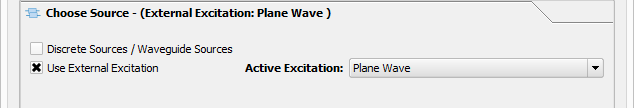
The  Choose Source tab is available only when a project utilizes at least one external excitation or static voltage point. Within the tab, users can choose one or both of the two available options: Discrete Sources and Use External Excitation.
Checking the Discrete Sources / Waveguide Sources option activates cell edges on which the electric field is modified using an input waveform to behave as a voltage or current source, such as a circuit component, modal waveguide interface, or nodal waveguide interface.
Checking the Use External Excitation option enables the Active Excitation setting, allowing users to choose from the project's external excitations. Only one type of external excitation can be active at a time, so users can select which plane wave to use for each calculation.
Set Up Parameter Sweeps
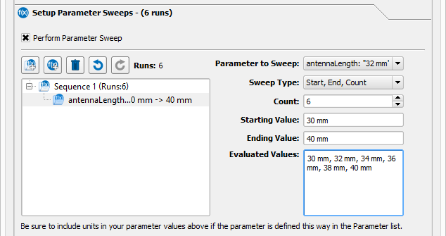
Setting up a parameter sweep is one of three basic steps that must be completed in order to run a parameter sweep. The  Setup Parameter Sweeps tab settings are enabled by checking the Perform Parameter Sweep option. These settings determine how a calculation sweeps through a single parameter or group of parameters.
The controls on the left side of the tab arrange parameter sweeps into groups, or sequences, and displays each parameter with a summary of values that specify the points at which a calculation is run. These values are determined by the settings on the right side of the tab.
Sequences and parameter sweeps are added and removed using the buttons above the window:
 : adds a new sequence.
  : adds a new parameter sweep to the selected sequence.
 : deletes the selected parameter sweep or sequence.
 : undoes the last action by reverting the tab's most recently changed setting to its previous value.
 : redoes the last undone action.
A sequence is considered invalid until a parameter is selected, enabling the remaining fields.
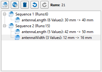
The controls on the right side of the tab determine what values each parameter is swept over. These specifications are summarized for each parameter displayed in the left window. Each parameter sweep is listed with its number of evaluated values in parentheses. The product of these values is displayed as the number of runs in parentheses following each sequence. The sum of these runs, or total number of calculations run in a simulation, appears as the Runs value above the window.
Multiple sequences can be defined for a single parameter and one sequence can contain a sweep of multiple parameters, so numerous calculations can be run during one simulation.
The Parameter to Sweep drop-down menu includes the available parameters from the parameters window. The selected parameter is swept according to the specified values that appear below, which must include units when the parameter is defined with units in the parameters window.
The Sweep Type drop-down menu provides three options for defining the input values. This selection determines which other settings must be specified.
- Start, Incr., Count: defines evenly spaced values that begin at the starting value, occur at each increment, and continue until the count number is fulfilled.
- Start, End, Count: defines evenly spaced values by dividing the space between the starting and ending values by the count value.
- Comma Separated: allows users to define each value, separated by a comma.
The additional specifications are used to define the parameter's set of values:
- Count: determines the number of values contained in a set, when applicable.
- Starting Value: determines the first value in a set. This value is the point at which the set begins.
- Increment: determines the space between each value in a set.
- Ending Value: determines the last value in a set. This value is the point at which the set ends.
- Input Values: user-defined values with no starting, ending, increment, or count value restrictions. The entered values must be separated by a comma.
The Evaluated Values display the complete set of parameter values, as defined by the fields above.
Set Up S-Parameters
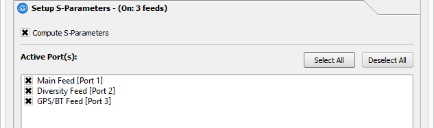
The  Setup S-Parameters tab is used for circuit components and waveguide interfaces. Checking the Compute S-Parameters option enables the Active Port(s) window that lists the project's defined ports. In a project with multiple ports defined, users can select any combination of ports or modes for circuit components or modal waveguide interfaces, respectively. Simulations with nodal waveguide interfaces require all pins to be selected. Each specified parameter sweep is performed for each active port.
The calculation for each active port provides data for one column of the S-parameter matrix. For example, selecting port one produces S11, S21, and S31 data for a three-port device. All ports must be selected in order to provide the full S-parameter matrix.
To calculate S-parameters, the simulation considers one port active at a time and sets each inactive port to its passive load equivalent. XF saves each calculation as one run in the same simulation, with each run differentiated by its active port number.
When Compute S-Parameters is unchecked, each port is active according to the power specified in its definition.

When collecting S-parameters with a nodal waveguide interface, the tab includes a Renormalization Impedance setting. This value is used in a modal to nodal conversion resulting in an impedance mismatch at the interface.

When specific absorption rate (SAR) averaging is enabled, the tab includes a SAR Averaging setting with options to compute SAR averaging for each active port or during post-processing only.
Frequencies of Interest
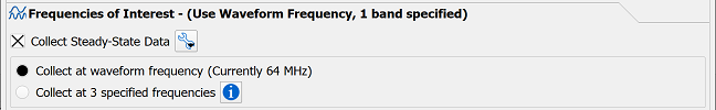
The  Frequencies of Interest tab allows users to specify what steady-state frequency data to collect during simulation. Near field and far field sensors defined in the project tree do not include a frequency, so users must specify one or more frequencies when creating the simulation. Checking the Collect Steady-State Data setting enables options for specifying frequencies as applicable to the current project, as well as the adjacent tool button.
The Collect at waveform frequency setting applies to simulations excited by a sinusoid waveform and saves steady-state data at the sinusoid frequency. For simulations excited by a broadband waveform, users can enter multiple steady-state frequencies by choosing the Collect at specified frequencies option and entering the desired values in the frequencies tab below.
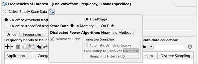
Clicking the tool button's drop-down arrow opens the DFT Settings, providing additional control over how steady-state data is generated. The FDTD solver converts the time domain results into frequency domain results when requested, and the temporary variables used to accomplish that must be stored.
The Store Data setting provides two options for storing data:
- In Memory: stores temporary data for the steady-state computations in memory.
- On Disk: stores temporary data for the steady-state computations in a file.
The default In Memory selection requires more memory than the On Disk option, but is also significantly faster. The On Disk selection reduces memory requirements to a manageable level when an insufficient amount of RAM is available, but reduces simulation speed due to file reading and writing.
The Dissipated Power Algorithm setting provides two options for determining dissipated power:
- Far-field Method: computes dissipated power by subtracting the power radiated through the outer boundaries of the simulation space from the net input power due to discrete components and waveguides.
- Near-field Method: computes dissipated power by summing the losses on all Yee-cell edges in the simulation space.
The Normalize Fields setting only applies when using a broadband excitation. Checking this option adjusts the steady-state field data to the same level of available power, similar to using a sinusoidal source at each frequency. This ensures agreement between steady-state results computed from a broadband and sinusoid waveform.
The Use Frequency-Dependent Material Properties on Nondispersive Materials setting applies when processing results for multiple steady-state frequencies. Checking this option converts dispersive material properties to their equivalent permittivity, permeability, and conductivity at each requested frequency. This affects results including dissipated power, SAR, and magnetic flux.
A running discrete Fourier transform (DFT) is used to compute steady-state fields from a broadband excitation. The Time Sampling group sets the DFT sampling interval and should be chosen to reduce aliasing. The Automatic Sampling Interval setting analyzes the frequency content of the input waveform and the requested steady-state frequencies to generate a sampling interval.
De-selecting this option enables the manual controls that determine the timestep sampling:
- Frequency to Resolve: highest possible frequency to analyze.
- Sampling Interval: specifies how often to sample the time-domain in timesteps.
These controls are interdependent, so entering one value also adjusts the other. The altered values are still editable and can be changed to the desired frequency and timestep.
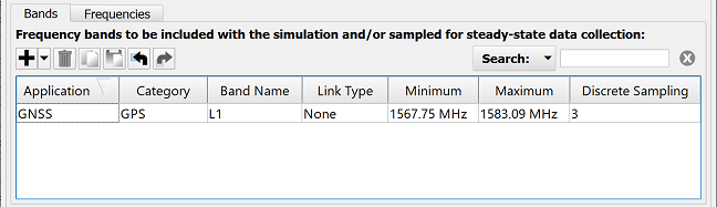
The Bands tab allows users to manage the frequency bands included with the simulation, as well as those sampled for steady-state data collection.
Bands are specified and removed using the buttons above the window:
 : adds a frequency band from the band library. The adjacent drop-down arrow provides the additional option to add an editable field for a user-defined frequency band.
- : removes the selected frequency bands from the window.
 : copies the selected frequency bands from the list.
 : pastes copied frequency bands into the list.
 : imports a band list from a previously exported *.rfb (Remcom Frequency Bands) file.
  : exports selected bands to an *.rfb (Remcom Frequency Bands) file.
On the right side of the tab, users can manually enter text into the Search field and use the drop-down arrow to access additional filtering criteria.
The Search Type determines what search terminology is considered valid:
- Simple: default search for case insensitive text matches, which are displayed as terms are entered.
- Regular Expression: case insensitive search for multiple terms separated by a vertical bar without spaces, and followed by pressing Enter. For example, band 1|system.
When choosing the Regular Expression search, users should note that entering a space either before or after a vertical bar returns incomplete search results. The Search These Fields options specify which fields are searched for the terms entered in the Search bar. The available selections include fields with either numeral or text entries, such as Application, Category, Band Name, and Link Type.
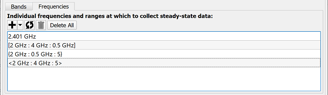
The Frequencies tab allows users to manage the individual frequencies and ranges at which to collect steady-state data.
Frequencies are specified and removed using the buttons above the window:
- : adds an editable field for a user-defined frequency. The adjacent drop-down arrow allows users to add a frequency list from the available options, or select Save current list to store the current set of entered frequencies as a list. The stored list appears only in this tab's drop-down menu.
 : replaces all entered frequencies with the selected frequency list, and includes a Save current list option to store the current set of entered frequencies as a list. The stored list appears only in this tab's drop-down menu.
- : removes the selected frequency from the window.
- Delete All: removes all entered frequencies from the window.
A single frequency is defined in each editable field, or a range of frequencies is entered using the following syntax:
- [start-value : end-value : increment]
- {start-value : increment : count}
- <start-value : end-value : count>
Specify the Field Formulation
The  Specify Field Formulation tab is available when a plane wave source is chosen to excite the simulation space. XF supports both the total-field/scattered-field simulation technique and the pure scattered field technique.
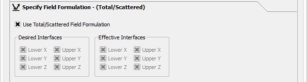
Checking the Use Total/Scattered Field Formulation option applies the total-field scattered-field formulation, which is preferable and more accurate in most cases. When using the total-field/scattered-field technique, the total E- and H-fields are simulated in the portion of the simulation space that contains the geometry, but only scattered E- and H-fields are simulated near the boundaries. Using a total-field/scattered-field plane wave source in conjunction with periodic boundary conditions enables the interface controls containing two sets of lower and upper x, y, and z boundaries.
The Desired Interfaces section specifies on which sides of the simulation space to include the total-field/scattered-field interface. These definitions might not be applicable due to the outer boundary conditions, or must be applied in conjunction with other definitions. Because the desired selections might not be applied, the uneditable Effective Interfaces section displays the actual definitions applied during the calculation.
Unchecking the Use Total/Scattered Field Formulation applies the pure scattered-field technique to the simulation, in which the scattered E- and H-fields are simulated over the full FDTD mesh.
Static Solver
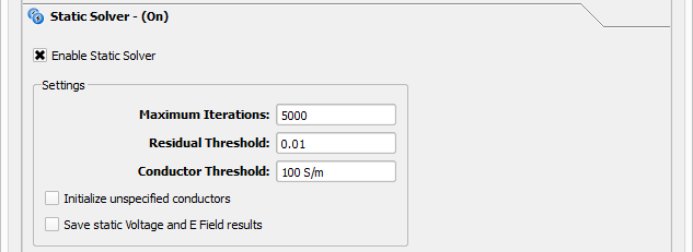
The  Static Solver tab is available for projects with one or more static voltage points defined, and it allows users to initialize the simulation with static electric fields by checking the Enable Static Solver setting. When this option is de-selected, all defined static voltage points are ignored during simulation.
Once the static solver is enabled, its criteria is set using the following editable fields:
- Maximum Iterations: greatest number of repetitions the solver will compute before terminating, regardless of whether or not it reaches the residual threshold.
- Residual Threshold: the value at which the static solver converges. Decreasing this target value increases the static solution's accuracy at the cost of computation time.
- Conductor Threshold: the conductivity at which the static solver defines a material as a good conductor.
When checked, the Initialize unspecified conductors option assigns a constant static voltage to unspecified conductors as well as conductors in contact with a static voltage point. Each specified conductor is assigned the voltage of the static voltage point to which it is electrically connected, and each unspecified conductor is assigned a voltage of zero. The static solver uses these initial values to calculate the surrounding electrostatic fields.
When unchecked, this option applies no value to an unspecified conductor and its voltage is calculated by the static solver using the initial values of specified conductors.
When checked, the Save static Voltage and E Field results option saves the calculated static voltage and electrostatic fields for viewing and post-processing. When this option is unchecked, the electrostatic fields initialize the simulation but are unavailable once the simulation has concluded.
Specify the Termination Criteria
Conceptually, the solver performs a number of computations before ending at a set maximum. Varying project contents and timestep durations demand more specific criteria for terminating a simulation. In the  Specify Termination Criteria tab, users can set conditions that give simulations a chance to reach convergence while limiting run time.
In a broadband calculation, convergence is reached when all electromagnetic energy dispates to zero. Due to numerical noise in the calculation, a nominal amount of electromagnetic energy often remains after convergence is reached. The threshold dictates when the calculation's value is acceptable enough to assume convergence.
In a sinusoid calculation, convergence is reached when near-zone data shows a constant amplitude sine wave, meaning all transient frequencies have subsided and the only remaining variation is sinusoidal.
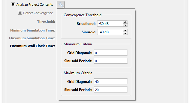
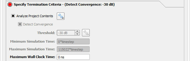
The Analyze Project Contents setting provides a project-based method for terminating the simulation. When this option is checked, XF calculates the disabled Threshold, Minimum Simulation Time, and Maximum Simulation Time based on the project's contents. These default values are appropriate in most cases, but can be modified using the adjacent drop-down settings.
The Convergence Threshold appears in the additional settings, and is separated into values for Broadband and Sinusoid waveforms. One of these two values is chosen based on the simulation's active waveforms and it appears in the tab's disabled Threshold field. A lower convergence value equates to more timesteps and a longer simulation, but produces more accurate results.
The Minimum Criteria options set the lowest number of timesteps the simulation must complete, regardless of whether or not it has reached the convergence threshold. One of these two values is chosen based on the simulation's active waveforms and it appears in the tab's disabled Minimum Simulation Time field.
The Maximum Criteria options set the number of timesteps the simulation must not exceed, regardless of whether or not it has reached the convergence threshold. One of these two values is chosen based on the simulation's active waveforms and it appears in the tab's disabled Maximum Simulation Time field.
These sections each contain a Grid Diagonals setting and a Sinusoid Periods setting for broadband and sinusoid waveforms, respectively.
These options determine the amount of time a simulation can run:
- Grid Diagonals: number of times the signal propagates to the corner located diagonally across the grid. This value uses the extent of the simulation space to define time.
- Sinusoid Periods: number of sinusoidal periods. This value uses the period of the waveform to define time.
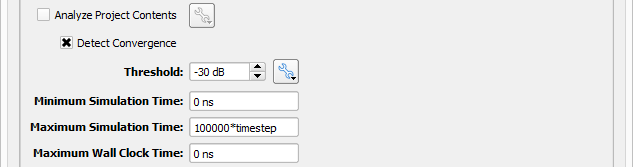
Unchecking the Analyze Project Contents option enables the tab's other settings. The Detect Convergence setting determines when convergence is reached using a method that is dependent upon the active waveform. Selecting this option enables both the Threshold and Minimum Simulation Time fields.
The editable Threshold field displays the Convergence Threshold for the appropriate waveform and provides additional convergence settings. Flatline Detection stops the calculation if a slow convergence is detected, even when the maximum number of timesteps has not been reached. This option applies when using the Detect Convergence setting with a broadband waveform.
The Spatial Sampling Density drop-down menu allows users to choose the amount of spatial samples used to determine convergence. The sampling density of the Low, Medium, and High settings range from every fourth point in each dimension to every point in each dimension. This option applies to both broadband and sinusoidal excitations.
The Temporal Sampling Interval controls the interval at which convergence is tested during calculations with broadband excitations.
The Sampling Periods setting is used only with a sinusoidal excitation.
The Minimum Simulation Time is the least amount of time a simulation must run before terminating, regardless of whether or not convergence is reached.
The Maximum Simulation Time is the greatest number of timesteps a simulation can run before terminating, regardless of whether or not convergence is reached. This setting is enabled any time the Analyze Project Contents option is deselected.
The Maximum Wall Clock Time is the amount of time elapsed from the start of the simulation to the time it is complete. Once this amount of time has passed, the simulation is terminated. This setting is enabled regardless of the Analyze Project Contents and Detect Convergence selections.
Notes
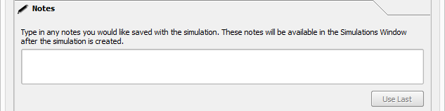
The  Notes tab provides space for users to attach memos to the simulation, such as a brief description of its specifications for later reference. When a note was attached to a previous project, the Use Last button is enabled and allows users to apply that same note to the current simulation setup. Once the simulation is created, these optional notes appear in the notes tab of the simulations window, and are editable in that window by right-clicking on the desired simulation and selecting from the menu.
Create and Queue
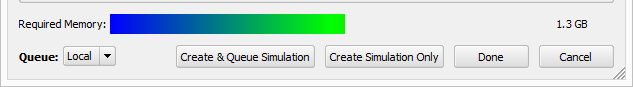
Before finalizing the simulation setup, users can verify the estimated total amount of memory required for the simulation using the Required Memory indicator and its corresponding value on the right side of the window. Mousing over the indicator displays additional information, such as the minimum and maximum usage values based on the current grid settings and requested results.
The Queue drop-down menu allows users to choose where to run the simulation, such as the local machine or a cluster.
Four buttons provide options for completing the simulation setup:
- Create & Queue Simulation: writes the input files to disk and queues the simulation to run.
- Create Simulation only: writes the input files to disk but does not queue the simulation.
- Done: closes the Create FDTD Simulation window and saves the entered specifications, which are visible when the window is re-opened.
- Cancel: closes the Create FDTD Simulation window but does not save the entered specifications.
The Create FDTD Simulation window closes once users make the final selection, and created simulations appear in the Simulations window.